
Mastering Numerical Methods For Partial Differential Equations with MATLAB
Event Date:
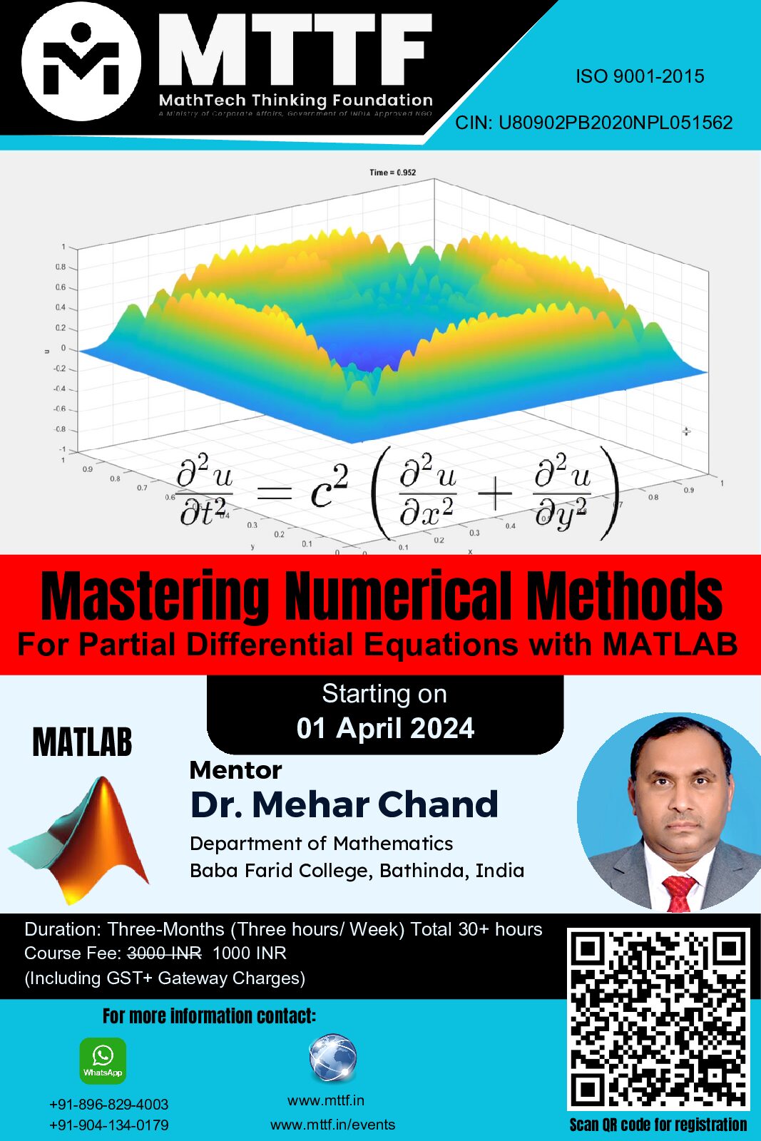
April 1, 2024
Event Time:
7:00 pm
Event Description
Key Information:
Registration Fee: 3000 INR 1000 INR (For all)
Starting on: 01 April 2024
Duration: 30 + Hours (3 Hours/ Week)
To Register Click on the buttonProgram Overview:
The “Mastering Numerical Methods for PDEs with MATLAB” course is meticulously crafted to furnish participants with profound comprehension and hands-on proficiency in tackling partial differential equations (PDEs) through MATLAB. Spanning 12 weeks, this course encompasses a diverse spectrum of numerical methodologies, ranging from classical techniques like Finite Difference, Finite Element, and Finite Volume methods to advanced strategies such as Spectral Methods, Galerkin Methods, and Wavelet Methods. Participants will engage in practical implementation of these methods using MATLAB, enabling them to effectively address intricate mathematical models prevalent in engineering, physics, and computational mathematics domains. This course harmoniously blends theoretical underpinnings with real-world applications, culminating in a course project where participants will employ acquired methods to solve a genuine PDE problem. With a dual focus on conceptual comprehension and practical implementation, this course is meticulously designed to empower participants with the requisite skills to proficiently navigate and master numerical methods for PDEs leveraging the versatile MATLAB platform.
About the course
- Comprehensive Content in PDF and Script Files: Participants will have access to detailed content in PDF files, ensuring a structured and easily accessible learning resource. Additionally, script files will be provided for hands-on practice and code implementation.
- Recording of Each Lecture: All lectures will be recorded, allowing participants to revisit and review the material at their own pace. This feature ensures that learners can reinforce their understanding of concepts and catch up on any missed sessions.
- Lifetime Access to Recordings and Content: Participants will enjoy lifetime access to both the recorded lectures and course content. This perpetual access ensures ongoing reinforcement of learning and serves as a valuable resource for future reference.
- Interactive Learning through Assignments and Quizzes: To enhance engagement and understanding, participants will be given assignments and quizzes. These interactive assessments provide an opportunity for hands-on application of concepts and reinforce theoretical knowledge.
- Flexibility in Learning: With recorded sessions and downloadable content, participants can learn at their own pace and revisit materials as needed. This flexibility accommodates diverse learning styles and schedules.
- Practical Implementation with Script Files: The provision of script files allows participants to directly engage in practical implementation of MATLAB solutions, reinforcing theoretical concepts through hands-on coding exercises.
- Comprehensive Coverage of Numerical Methods: The course ensures a thorough exploration of various numerical methods, providing participants with a diverse toolkit for solving ODEs and addressing real-world problems.
- Supportive Learning Environment: Assignments, quizzes, and recorded lectures contribute to a supportive and interactive learning environment. Participants can actively engage with the material, seek clarification, and apply their knowledge through practical assessments.
- Lifetime Learning Community: Participants become part of a lifetime learning community, fostering collaboration and networking opportunities with fellow learners and instructors.
Rationale for Partial Differential Equations (PDEs):
Partial differential equations (PDEs) serve as cornerstone elements in modeling and deciphering complex physical phenomena across diverse scientific disciplines. Unlike ordinary differential equations (ODEs), PDEs delineate the variations of functions and their derivatives concerning multiple independent variables, rendering them indispensable for scrutinizing systems rife with spatial and temporal dependencies. PDEs form the bedrock of physics, engineering, and applied mathematics, governing phenomena spanning heat conduction, fluid dynamics, electromagnetism, and quantum mechanics. Their extensive applicability stems from their adeptness in encapsulating continuous variations and interactions within systems, furnishing a robust framework for elucidating natural phenomena and engineering processes. Solving PDEs empowers prediction of behaviors, optimization of designs, and simulation of real-world scenarios, thereby catalyzing advancements in technology, medicine, and research. Furthermore, numerical methods tailored for PDEs, particularly when implemented via MATLAB, proffer efficient and precise approaches to grapple with complex problems that often elude analytical solutions, rendering them indispensable tools for scientists, engineers, and researchers alike.
Significance of Numerical Methods for PDEs:
Numerical methods devised for partial differential equations (PDEs) play a pivotal role in contemporary scientific and engineering landscapes, furnishing indispensable tools for unraveling intricate mathematical models characterizing dynamic physical phenomena. These methodologies furnish pragmatic solutions to quandaries devoid of analytical resolutions or burdened with computational intractability. By discretizing continuous PDEs into manageable systems, numerical methods facilitate exploration of diverse physical scenarios, enabling simulations of fluid dynamics, heat transfer, quantum mechanics, and more. Within the realm of computational mathematics, adept comprehension and implementation of these methodologies, particularly within the robust framework of MATLAB, empower researchers and practitioners to faithfully model real-world phenomena, prognosticate system behaviors, and optimize designs. This convergence bridges the chasm between theoretical formulations and practical applications across myriad scientific and engineering disciplines.
Target Audience:
Tailored for engineers, physicists, and computational mathematicians endeavoring to augment their prowess in solving partial differential equations (PDEs), this course proffers an ideal avenue for individuals yearning to cultivate comprehensive insights into numerical methodologies utilizing MATLAB. It equips participants with practical acumen requisite to navigate and address complex mathematical models pervasive in their respective fields.
Preliminaries:
Participants are anticipated to harbor foundational comprehension of PDEs and possess rudimentary proficiency in MATLAB. Familiarity with mathematical concepts germane to engineering and physics would be advantageous. This course is architected to build upon these preliminary prerequisites, furnishing in-depth knowledge and hands-on experience in mastering diverse numerical methods for PDE problem-solving leveraging MATLAB.
Additional Components:
- Interactive Sessions: Weekly live sessions for Q&A, problem-solving, and code walkthroughs.
- Assignments and Assessments: Regular assignments to reinforce learning and assess understanding.
- Resource Materials: Supplementary reading materials, code samples, and MATLAB scripts.
- Discussion Forums: Online forums for participants to collaborate, ask questions, and share insights.
Program Structure:
(1) Finite Difference Method (FDM): FDM discretizes partial differential equations by approximating derivatives with finite difference approximations, converting the continuous problem into a system of algebraic equations.
(2) Finite Element Method (FEM): FEM divides the domain into smaller, simpler elements, approximating the solution within each element using basis functions, and then assembling these elements to solve the entire problem.
(3) Finite Volume Method (FVM): FVM discretizes the domain by dividing it into control volumes, where the conservation laws are applied locally to each volume, representing fluxes across the control volume faces.
(4) Method of Lines (MOL): MOL discretizes the spatial domain while keeping the temporal dimension continuous, transforming the partial differential equation into a system of ordinary differential equations (ODEs) that can be solved using time-stepping methods.
(5) Explicit Euler Method: An explicit time-stepping method that approximates the solution of ordinary differential equations by taking a single forward step based on the current derivative.
(6) Implicit Euler Method: An implicit time-stepping method that involves solving a system of equations at each time step, including future values, making it more stable for stiff problems compared to explicit methods.
(7) Crank-Nicolson Method: A time-stepping method that combines the Implicit Euler and Explicit Euler methods, offering second-order accuracy by averaging the values at the current and future time steps.
(8) Upwind Scheme: A numerical scheme for advection-dominated problems that uses information from the upwind direction to determine the spatial derivative, ensuring stability by considering the direction of flow.
(9) Downwind Scheme: Similar to the upwind scheme, but uses information from the downwind direction for calculating spatial derivatives, appropriate for problems with dominant downstream flow.
(10) Leapfrog Method: A second-order accurate time-stepping method that updates the solution at each time step based on the values at the previous and next time steps, often used in wave propagation problems.
(11) Lax-Wendroff Method: A high-resolution numerical scheme that combines forward and backward differencing to achieve second-order accuracy in both space and time.
(12) MacCormack Method: A two-step predictor-corrector method used for solving time-dependent problems, involving a prediction step followed by a correction step to improve accuracy.
(13) Operator Splitting Method: A technique for splitting a complex PDE into simpler sub-problems, allowing separate treatment of each component, often used when the PDE has multiple terms with different characteristics.
(14) Spectral Methods: Numerical techniques that represent the solution using basis functions, such as Fourier series or Chebyshev polynomials, providing high accuracy by capturing global behavior of the solution.
(15) Chebyshev Collocation Method: A spectral method that approximates the solution using Chebyshev polynomials and collocation points, offering exponential convergence for smooth solutions.
(16) Galerkin Method: A variational method that seeks an approximate solution by minimizing the residual in a weighted integral sense, commonly used in the Finite Element Method.
(17) Boundary Element Method (BEM): A numerical technique that discretizes the boundary of the domain and solves integral equations to obtain the solution, particularly suited for problems with solutions satisfying the boundary conditions.
(18) Petrov-Galerkin Method: A variant of the Galerkin method where different trial and test functions are used, often chosen to improve stability or convergence properties.
(19) Semi-Lagrangian Method: A numerical technique for solving advection-dominated problems that traces characteristics backward in time to update the solution, offering unconditional stability.
(20) Adams-Bashforth Method: An explicit time-stepping method based on extrapolating the solution using previous values and derivatives, commonly used for initial value problems.
(21) Adams-Moulton Method: An implicit counterpart to the Adams-Bashforth method, involving backward extrapolation for better stability and accuracy.
(22) Runge-Kutta Methods: A family of explicit and implicit methods for solving ordinary differential equations by combining multiple stage calculations to improve accuracy.
(23) Moving Mesh Methods: Techniques that dynamically adjust the computational grid based on solution behavior, optimizing grid resolution in regions of interest and reducing computational cost.
(24) Meshfree Methods: Numerical techniques that do not require a fixed mesh, such as radial basis functions or moving least squares, offering flexibility in handling complex geometries and adaptivity.
(25) Wavelet Methods: Methods that represent the solution using wavelet basis functions, allowing for adaptive resolution and efficient representation of solutions with localized features.
Course Content:
(1) Introduction to Numerical Methods for PDEs: Overview of PDEs and their significance in scientific computing; Introduction to MATLAB for numerical computation
(2) Finite Difference Method (FDM): Principles of FDM and its applications in discretizing PDEs
Implementation of FDM in MATLAB for solving various types of PDEs
(3) Finite Element Method (FEM): Fundamentals of FEM and its advantages in solving complex PDEs;
Hands-on experience with FEM implementation in MATLAB
(4) Finite Volume Method (FVM): Understanding the concept of FVM and its applicability in practical problems; Implementation of FVM algorithms in MATLAB for solving PDEs with conservation laws
(5) Method of Lines (MOL): Introduction to MOL and its role in solving time-dependent PDEs; Practical implementation of MOL using MATLAB for transforming PDEs into ODE systems
(6) Explicit and Implicit Time-stepping Methods: Detailed explanation of explicit and implicit Euler methods; Implementation and comparison of explicit and implicit methods in MATLAB
(7) Crank-Nicolson Method and its Variants: Theory behind the Crank-Nicolson method and its advantages; Hands-on session on implementing Crank-Nicolson method in MATLAB
(8) Advanced Numerical Schemes for Advection-Dominated Problems: Detailed discussion on upwind and downwind schemes; Implementation of these schemes in MATLAB for advection-dominated PDEs
(9) High-Resolution Methods: Overview of leapfrog, Lax-Wendroff, and MacCormack methods
Practical implementation and comparison of these methods in MATLAB
(10) Spectral Methods and Variants: Understanding the principles of spectral methods and Chebyshev collocation method; Hands-on session on implementing spectral methods in MATLAB
(11) Galerkin Method and Boundary Element Method (BEM): Introduction to Galerkin and BEM for solving PDEs with boundary conditions; Implementation of Galerkin and BEM techniques in MATLAB
(12) Petrov-Galerkin Method and Semi-Lagrangian Method: Theory and practical implementation of Petrov-Galerkin and Semi-Lagrangian methods in MATLAB
(13) Time-stepping Methods: Adams-Bashforth, Adams-Moulton, and Runge-Kutta; Detailed explanation and implementation of various time-stepping methods in MATLAB
(14) Advanced Techniques: Moving Mesh Methods, Meshfree Methods, and Wavelet Methods; Overview and practical implementation of advanced numerical techniques in MATLAB